Using the `calibrate()` function for parameter estimation
Ricardo Oliveros-Ramos
2025-12-20
Source:vignettes/v02-parameter_estimation.Rmd
v02-parameter_estimation.RmdIntroduction
This vignette focus on the use of the calibrate() for
parameter estimation. We suggest to see the vignette ‘Getting started
with the calibrar package’ before reading this one,
specially if you do not have previous experience doing optimization in
R.
Estimating parameters for a linear model
As a first example, we will estimate the parameters for a linear
model by manually performing the optimization, in opposition of the
standard method using the stats::lm(). The objetive of this
is to introduce the features of the calibrate() function
with a simple and fast model. Let’s start by creating some parameters
for the linear model.
library(calibrar)
N = 7 # number of variables in the linear model
T = 100 # number of observations
sd = 0.25 # standard deviation of the gaussian noise
# observed data
x = matrix(rnorm(N*T, sd=sd), nrow=T, ncol=N)
# slopes for the linear model (real parameters)
slope = seq_len(N)
# intercept for the linear model (real parameters)
intercept = pi
# real parameters
real = list(intercept=intercept, slope=slope)
real
#> $intercept
#> [1] 3.141593
#>
#> $slope
#> [1] 1 2 3 4 5 6 7
Now, let’s create a function so simulate the linear model.
# function to simulate the linear model
linear = function(x, par) {
  stopifnot(length(x)==length(par$slope))
  out = sum(x*par$slope) + par$intercept
  return(out)
}
And, finally, the simulated data for the exercise:
# simulated data
y = apply(x, 1, linear, par=real)
Of course, the solution can be found using the lm()
function:
mod = lm(y ~ x)
mod
#>
#> Call:
#> lm(formula = y ~ x)
#>
#> Coefficients:
#> (Intercept)           x1           x2           x3           x4           x5
#>       3.142        1.000        2.000        3.000        4.000        5.000
#>          x6           x7
#>       6.000        7.000
Now, in order to proceed to find the solution by an explicit numerical optimization, we need to define the objective function to be minimized:
# objective function (residual squares sum)
obj = function(par, x, y) {
  y_sim = apply(x, 1, linear, par=par)
  out = sum((y_sim - y)^2)
  return(out)
}
So now we can proceed with the optimization:
# initial guess for optimization
start = list(intercept=0, slope=rep(0, N))
bfgs = calibrate(par=start, fn=obj, x=x, y=y)
#> Using optimization method 'Rvmmin'.
#> Elapsed time: 0.12s
#> Function value: 5.28185e-14
#> Parameter values: 3.14 1 2 3 4 5 6 7
#>
#> Status: Rvmminu appears to have converged
# using coef to extract optimal parameters
coef(bfgs)
#> $intercept
#> [1] 3.141593
#>
#> $slope
#> [1] 1 2 3 4 5 6 7
As expected, we were able to recover the real parameters of the
model. Now, let’s specify lower and upper
bounds for the algorithms that require them:
And repeat the exercise with several optimization algorithms:
set.seed(880820) # for reproducibility
cg = calibrate(par=start, fn=obj, x=x, y=y, method='CG')
#> Using optimization method 'CG'.
#> Elapsed time: 0.42s
#> Function value: 3.37729e-13
#> Parameter values: 3.14 1 2 3 4 5 6 7
#>
#> Status: -
nm = calibrate(par=start, fn=obj, x=x, y=y, method='nmkb', lower=lower, upper=upper)
#> Using optimization method 'nmkb'.
#> Elapsed time: 0.28s
#> Function value: 5.28315e-07
#> Parameter values: 3.14 1 2 3 4 5 6 7
#>
#> Status: -
ahres = calibrate(par=start, fn=obj, x=x, y=y, method='AHR-ES')
#> Using optimization method 'AHR-ES'.
#> Elapsed time: 1.47s
#> Function value: 2.66292e-18
#> Parameter values: 3.14 1 2 3 4 5 6 7
#>
#> Status: Stopping criteria reached in 234 generations.
hjn = calibrate(par=start, fn=obj, x=x, y=y, method='hjn', lower=lower, upper=upper)
#> Using optimization method 'hjn'.
#> Elapsed time: 0.38s
#> Function value: 2.15391e-13
#> Parameter values: 3.14 1 2 3 4 5 6 7
#>
#> Status: hjn appears to have converged
And compare the results:
summary(ahres, hjn, nm, bfgs, cg, par.only=TRUE)
#>       method intercept slope1 slope2 slope3 slope4 slope5 slope6 slope7
#> ahres AHR-ES      3.14      1      2      3      4      5      6      7
#> hjn      hjn      3.14      1      2      3      4      5      6      7
#> nm      nmkb      3.14      1      2      3      4      5      6      7
#> bfgs  Rvmmin      3.14      1      2      3      4      5      6      7
#> cg        CG      3.14      1      2      3      4      5      6      7
As we can see, for this simple example, all the algorithms used were able to find the solution within a reasonable time, but some were faster than others. In the next examples we will see this is not always the case, and some algorithms can perform very differently or even fail for a particular optimization problem.
Fitting a biomass production model with harvest
As a second example, we will estimate the parameters for a difference equation system, simulating the dynamics of the biomass B of a harvested population:
B_{t+1} = B_t + rB_t\left(1-\frac{B_t}{K}\right) - C_t, where B_t is the biomass in time t, C_t is the catch during the interval [t, t+1[, r is the intrinsic population growth rate and K is the carrying capacity of the system.
We will define some values for all the parameters so we can perform an optimization an try to recover them from the simulated data:
set.seed(880820)
T = 50
real = list(r=0.5, K=1000, B0=600)
catch = 0.25*(real$r*real$K)*runif(T, min=0.2, max=1.8)
As before, a function to simulate data from the parameters (the
model) will be needed. The requirement for this function is to have as
first argument the parameter vector (or list) par:
run_model = function(par, T, catch) {
  B = numeric(T+1)
  times = seq(0, T)
  B0 = par$B0
  r = par$r
  K = par$K
  B[1] = B0
  for(t in seq_len(T)) {
    b = B[t] + r*B[t]*(1-B[t]/K) - catch[t] # could be negative
    B[t+1] = max(b, 0.01*B[t]) # smooth aproximation to zero
  }
  out = list(biomass=B)
  return(out)
}
And now we can use the run_model() function and the
assumed parameters to simulate the model:
observed = run_model(par=real, T=T, catch=catch)
par(mfrow=c(2,1), mar=c(3,3,1,1), oma=c(1,1,1,1))
plot(observed$biomass, type="l", lwd=2, ylab="biomass", xlab="", las=1, ylim=c(0, 1.2*max(observed$biomass)))
mtext("BIOMASS", 3, adj=0.01, line = 0, font=2)
plot(catch, type="h", lwd=2, ylab="catch", xlab="", las=1, ylim=c(0, 1.2*max(catch)))
mtext("CATCH", 3, adj=0.01, line = 0, font=2)
In order to carry out the optimization, we need the objective function to be defined, in this case, using a simple residual squares sum:
objfn = function(par, T, catch, observed) {
  simulated = run_model(par=par, T=T, catch=catch)
  value = sum((observed$biomass-simulated$biomass)^2, na.rm=TRUE)
  return(value)
}
Finally, we need to define a starting point for the search,
and we are ready to try to estimate the parameters using several algorithms:
set.seed(880820) # for reproducibility
opt0 = calibrate(par=start, fn = objfn, method='LBFGSB3', T=T, catch=catch, observed=observed)
#> Using optimization method 'LBFGSB3'.
#> Elapsed time: 0.09s
#> Function value: 150998
#> Parameter values: 0.402 1.18e+03 600
#>
#> Status: CONVERGENCE: Parameters differences below xtol
opt1 = calibrate(par=start, fn = objfn, method='Rvmmin', T=T, catch=catch, observed=observed)
#> Using optimization method 'Rvmmin'.
#> Elapsed time: 0.02s
#> Function value: 1.34546e+07
#> Parameter values: 2.9 1.14e+03 482
#>
#> Status: Rvmminu appears to have converged
opt2 = calibrate(par=start, fn = objfn, method='CG', T=T, catch=catch, observed=observed)
#> Using optimization method 'CG'.
#> Elapsed time: 0.08s
#> Function value: 150931
#> Parameter values: 0.402 1.18e+03 600
#>
#> Status: -
opt3 = calibrate(par=start, fn = objfn, method='AHR-ES', T=T, catch=catch, observed=observed)
#> Using optimization method 'AHR-ES'.
#> Elapsed time: 1.81s
#> Function value: 6.77545e-17
#> Parameter values: 0.5 1e+03 600
#>
#> Status: Stopping criteria reached in 1590 generations.
opt4 = calibrate(par=start, fn = objfn, method='CMA-ES', T=T, catch=catch, observed=observed)
#> Using optimization method 'CMA-ES'.
#> Elapsed time: 0.09s
#> Function value: 107373
#> Parameter values: 0.446 1.09e+03 689
#>
#> Status: Covariance matrix 'C' is numerically not positive definite.
opt5 = calibrate(par=start, fn = objfn, method='hjn', T=T, catch=catch, observed=observed)
#> Using optimization method 'hjn'.
#> Elapsed time: 0.38s
#> Function value: 990.8
#> Parameter values: 0.509 988 602
#>
#> Status: Function count limit exceeded.
opt6 = calibrate(par=start, fn = objfn, method='Nelder-Mead', T=T, catch=catch, observed=observed)
#> Using optimization method 'Nelder-Mead'.
#> Elapsed time: 0.01s
#> Function value: 0.0775804
#> Parameter values: 0.5 1e+03 600
#>
#> Status: -
The function summary() can be used to compare all the
optimization results:
summary(opt0, opt1, opt2, opt3, opt4, opt5, opt6)
#>           method elapsed    value    fn  gr     r    K  B0
#> opt0     LBFGSB3  0.0903 1.51e+05    18  18 0.402 1181 600
#> opt1      Rvmmin  0.0162 1.35e+07   161   8 2.900 1145 482
#> opt2          CG  0.0804 1.51e+05   691 101 0.402 1181 600
#> opt3      AHR-ES  1.8073 6.78e-17 11130   0 0.500 1000 600
#> opt4      CMA-ES  0.0866 1.07e+05  1085  NA 0.446 1090 689
#> opt5         hjn  0.3836 9.91e+02  6000  NA 0.509  988 602
#> opt6 Nelder-Mead  0.0128 7.76e-02   221  NA 0.500 1000 600
For a better comparison, we can simulate the results for all the parameters found:
sim0 = run_model(par=coef(opt0), T=T, catch=catch)
sim1 = run_model(par=coef(opt1), T=T, catch=catch)
sim2 = run_model(par=coef(opt2), T=T, catch=catch)
sim3 = run_model(par=coef(opt3), T=T, catch=catch)
sim4 = run_model(par=coef(opt4), T=T, catch=catch)
sim5 = run_model(par=coef(opt5), T=T, catch=catch)
And plot some of the best results obtained (L-BFGS-B 3.0, CG and AHR-ES):
par(mar=c(3,4,1,1))
plot(observed$biomass, type="n", ylab="BIOMASS", xlab="", las=1, ylim=c(0, 1.2*max(observed$biomass)))
lines(sim0$biomass, col=1, lwd=2)
lines(sim2$biomass, col=2, lwd=2)
lines(sim3$biomass, col=3, lwd=2)
points(observed$biomass)
mtext(c('LBFGSB3', 'CG', 'AHR-ES'), 1, adj=0.05, col=1:3, line=-(4:2), font=2)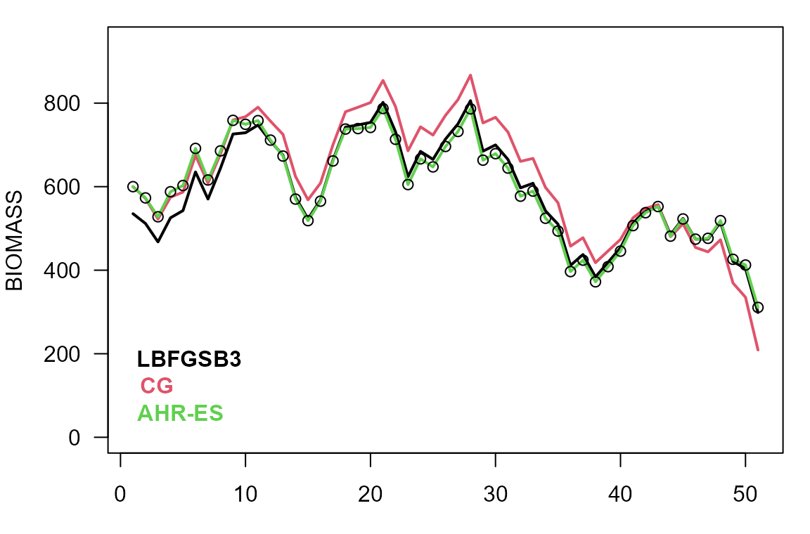
So far, we have used all algorithms with their default arguments.
Most algorithms provide control arguments that allow to improve its
performance for a particular problem. For example, looking back to the
results from the L-BFGS-B 3.0 method, we can see as status ‘Maximum
number of iterations reached’, meaning the algorithm did not converge
but stopped after the maximum number of 100 iterations allowed by
default. This can be modified here (and for several other methods) by
changing the maxit control argument:
optx = calibrate(par=start, fn = objfn, method='LBFGSB3', T=T, catch=catch, observed=observed, control=list(maxit=20000))
#> Using optimization method 'LBFGSB3'.
#> Elapsed time: 0.01s
#> Function value: 150998
#> Parameter values: 0.402 1.18e+03 600
#>
#> Status: CONVERGENCE: Parameters differences below xtol
And we can see that with this setup, the algorithm converges to the right solution.
We also have the possibility to set up a calibration in multiple phases, meaning we will solve several sequential optimizations with a progressively higher number of parameters. The purpose of this is to improve the initial search point for a final optimization with all the parameters active. This heuristic may help to achieve find the solution for some problems. For example, the Rvmmin algorithm has a status ‘Rvmminu appears to have converged’ but was not able to converge to the original parameter values. So, we will try again by fixing some of the parameters (the initial biomass) and trying a two phases parameter estimation:
calibrate(par=start, fn = objfn, method='Rvmmin', T=T, catch=catch, observed=observed, phases = c(1,1,2))
#> Parameter estimation in two phases.
#>
#> - Phase 1: 2 out of 3 parameters are currently active.
#>  Using optimization method 'Rvmmin'.
#>  Phase 1 finished (0.01s)
#>  Function value: 1.8303e-08
#>  Parameter values: 0.5 1e+03
#>
#> - Phase 2: 3 out of 3 parameters are currently active.
#>  Using optimization method 'Rvmmin'.
#>  Phase 2 finished (0.00s)
#>  Function value: 1.8303e-08
#>  Parameter values: 0.5 1e+03 600
#>
#> Status: Rvmminu appears to have converged
#> Optimization using 'Rvmmin' algorithm.
#> Function value: 1.830304e-08
#> Status: Rvmminu appears to have converged
#> Parameters:
#>     r     K    B0
#> 5e-01 1e+03 6e+02
#> Computation:
#> function gradient
#>       18        1
And with two phases, now we also find the solution using the ‘Rvmmin’ method.
Fitting an autoregressive Poisson model
As a third example, we will estimate the parameters for a Poisson Autoregressive Mixed model for the dynamics of a population in different sites:
log(\mu_{i, t+1}) = log(\mu_{i, t}) + \alpha + \beta X_{i, t} + \gamma_t
where \mu_{i, t} is the size of the
population in site i at year t, X_{i, t}
is the value of an environmental variable in site i at year t.
The parameters to estimate were \alpha,
\beta, and \gamma_t, the random effects for each year,
\gamma_t \sim N(0,\sigma^2), and the
initial population at each site \mu_{i,
0}. We assumed that the observations N_{i,t} follow a Poisson distribution with
mean \mu_{i, t}. We could also create
the data for this model using the function calibrar_demo(),
with the additional arguments L=5 (five sites) and
T=100 (one hundred years):
path = NULL # NULL to use the current directory
ARPM = calibrar_demo(path=path, model="PoissonMixedModel", L=5, T=100)
#> Creating observed data list for calibration...
#> Loaded observed data for variables: 'site_1', 'site_2', 'site_3', 'site_4', 'site_5'.
setup = calibration_setup(file=ARPM$setup)
observed = calibration_data(setup=setup, path=ARPM$path)
#> Creating observed data list for calibration...
#>
#> Loaded observed data for variables: 'site_1', 'site_2', 'site_3', 'site_4', 'site_5'.
forcing = as.matrix(read.csv(file.path(ARPM$path, "master", "environment.csv"), row.names=1))
control = list(maxit=20000, eps=sqrt(.Machine$double.eps), factr=sqrt(.Machine$double.eps))
Here, we also added a control list to increase the
maximum number of iterations for the algorithms and the tolerance for
the convergence. Now we can specify the run_model()
function so we can simulate the model from a parameter set and define
the objective function using the calibration_objFn()
function:
run_model = function(par, forcing) {
  output = calibrar:::.PoissonMixedModel(par=par, forcing=forcing)
  output = c(output, list(gammas=par$gamma)) # adding gamma parameters for penalties
  return(output)
}
obj = calibration_objFn(model=run_model, setup=setup, observed=observed, forcing=forcing, aggregate=TRUE)With these we can proceed to the parameter estimation. Here, we will compare the performance of three BFGS type algorithms:
# real parameters
coef(ARPM)
#> $alpha
#> [1] 0.4
#>
#> $beta
#> [1] -0.4
#>
#> $gamma
#>  [1] -0.1252736456  0.0962670651  0.3390542168 -0.3522452588  0.0396026030
#>  [6]  0.0794698198  0.0058450990  0.5120546777  0.2514255423 -0.1069075371
#> [11] -0.1250454857  0.1827697374  0.2014399069  0.1438583647 -0.1209423322
#> [16]  0.1078108813 -0.0153661771  0.3699839121 -0.1709815103  0.0065274590
#> [21] -0.2050118962 -0.1964498151  0.0008203914 -0.0466854356 -0.0997776438
#> [26]  0.3099425926  0.0174993833  0.2637402261 -0.1962448238 -0.0491245175
#> [31] -0.2807867674  0.2881786295 -0.1962719982  0.2948489808 -0.1982394491
#> [36] -0.0188994689 -0.5750283368 -0.0493732202  0.0029488980 -0.3838175407
#> [41] -0.0575627487 -0.0693274891 -0.3679177169  0.1797177882 -0.2425710022
#> [46] -0.0437928463  0.1128536321 -0.1050868751  0.1488748450  0.0257963506
#> [51]  0.2976548514 -0.1325363902 -0.2321310003  0.0717548469 -0.0389692768
#> [56] -0.0590564016  0.0993280847  0.0969825576  0.0037569001  0.1269549129
#> [61]  0.1508888175  0.1667178070  0.1931522592  0.2587759936 -0.0273102042
#> [66] -0.0880277376 -0.2454567829 -0.0475306139 -0.1853716313  0.0822470712
#> [71] -0.0397729154 -0.1114899279 -0.1954314245  0.0121470497 -0.1194458959
#> [76] -0.2517897395 -0.2820094403  0.2202608159 -0.1354484053 -0.1524347015
#> [81] -0.0583497204 -0.1150377059 -0.0887883736 -0.0625140888 -0.1206008853
#> [86] -0.2187869440  0.1429412383 -0.0217624526 -0.2887595871  0.1612246527
#> [91] -0.3479670157 -0.0802640619 -0.0575164978 -0.1876814800  0.0575334278
#> [96] -0.3010802249  0.3038594027  0.0734818712  0.3399724818
#>
#> $sd
#> [1] 0.2
#>
#> $mu_ini
#> [1] 5.141664 4.158883 3.433987 4.430817 4.934474
lbfgsb1 = calibrate(par=ARPM$guess, fn=obj, method='L-BFGS-B', lower=ARPM$lower, upper=ARPM$upper, phases=ARPM$phase, control=control)
#> Using optimization method 'L-BFGS-B'.
#> Elapsed time: 1m 0.1s
#> Function value: -186093
#> Parameter values: 0.43 -0.415 -0.109 0.103 0.224 -0.306 0.0191 0.0445 0.0534 0.432 0.199 -0.0786 -0.128 0.121 0.275 0.0471 -0.101 0.0981 -0.0389 0.371 -0.213 0.036 -0.237 -0.254 0.0572 -0.0642 -0.178 0.294 5.54e-05 0.268 -0.212 -0.0516 -0.325 0.253 -0.195 0.291 -0.243 -0.0235 -0.532 -0.0742 -0.0616 -0.297 -0.115 -0.167 -0.323 0.0585 -0.185 -0.0309 0.0992 -0.0813 0.0103 0.161 0.266 -0.103 -0.368 0.0792 -0.133 0.0369 0.0815 -0.000515 0.0957 -0.0619 0.287 0.185 0.134 0.162 0.0492 -0.143 -0.124 -0.163 -0.277 0.0741 -0.0474 -0.0123 -0.229 -0.0587 -0.17 -0.183 -0.226 -0.0318 -0.0141 -0.21 -0.0744 -0.1 -0.185 -0.137 -0.0275 -0.164 0.181 -0.2 -0.243 0.152 -0.284 -0.352 -0.0418 -0.188 0.0203 -0.0106 0.197 -0.0425 0.37
#>
#> Status: CONVERGENCE: REL_REDUCTION_OF_F <= FACTR*EPSMCH
lbfgsb2 = calibrate(par=ARPM$guess, fn=obj, method='Rvmmin', lower=ARPM$lower, upper=ARPM$upper, phases=ARPM$phase, control=control)
#> Using optimization method 'Rvmmin'.
#> Elapsed time: 12.64s
#> Function value: -186095
#> Parameter values: 0.397 -0.415 -0.0755 0.135 0.261 -0.276 0.0524 0.0757 0.085 0.467 0.231 -0.0459 -0.0946 0.155 0.308 0.0794 -0.0678 0.131 -0.00842 0.405 -0.181 0.0701 -0.205 -0.221 0.0894 -0.0332 -0.145 0.326 0.0332 0.301 -0.179 -0.0193 -0.291 0.284 -0.161 0.323 -0.209 0.00885 -0.5 -0.0401 -0.0301 -0.27 -0.0754 -0.135 -0.295 0.0923 -0.154 0.00403 0.137 -0.0503 0.0357 0.194 0.307 -0.0752 -0.339 0.117 -0.101 0.0691 0.114 0.0343 0.129 -0.0325 0.325 0.217 0.164 0.197 0.0826 -0.113 -0.0906 -0.128 -0.25 0.111 -0.015 0.0211 -0.201 -0.0202 -0.134 -0.154 -0.195 0.0029 0.0188 -0.179 -0.0423 -0.0657 -0.151 -0.104 0.00175 -0.13 0.209 -0.167 -0.206 0.187 -0.246 -0.32 -0.00722 -0.145 3.35e-05 0.0373 0.242 0.00104 0.408
#>
#> Status: Rvmminb appears to have converged
lbfgsb3 = calibrate(par=ARPM$guess, fn=obj, method='LBFGSB3', lower=ARPM$lower, upper=ARPM$upper, phases=ARPM$phase, control=control)
#> Using optimization method 'LBFGSB3'.
#> Elapsed time: 40.27s
#> Function value: -186092
#> Parameter values: 0.417 -0.415 -0.0863 0.118 0.233 -0.279 0.00507 0.0474 0.0892 0.442 0.216 -0.0689 -0.116 0.136 0.294 0.0629 -0.0932 0.106 -0.0347 0.405 -0.202 0.0494 -0.232 -0.241 0.0753 -0.0617 -0.16 0.307 0.0214 0.287 -0.204 -0.053 -0.305 0.256 -0.16 0.303 -0.225 -0.0281 -0.501 -0.0754 -0.0467 -0.276 -0.0988 -0.155 -0.338 0.108 -0.205 -0.0232 0.139 -0.0669 0.0252 0.172 0.285 -0.0895 -0.377 0.132 -0.154 0.0467 0.0941 0.00561 0.129 -0.0686 0.317 0.194 0.161 0.182 0.0628 -0.129 -0.126 -0.151 -0.27 0.0967 -0.0474 0.0142 -0.223 -0.0329 -0.158 -0.161 -0.222 -0.00932 0.00186 -0.229 -0.0546 -0.0754 -0.173 -0.12 -0.00392 -0.177 0.223 -0.228 -0.26 0.227 -0.271 -0.348 0.00114 -0.184 0.031 -0.022 0.2 -0.0395 0.411
#>
#> Status: CONVERGENCE: Parameters differences below xtol
summary(ARPM, lbfgsb1, lbfgsb2, lbfgsb3, show_par = 1:3)
#>           method elapsed   value   fn   gr alpha   beta  gamma1
#> ARPM        data      NA -186178   NA   NA 0.400 -0.400 -0.1253
#> lbfgsb1 L-BFGS-B    60.1 -186093 2082 2082 0.430 -0.415 -0.1085
#> lbfgsb2   Rvmmin    12.6 -186095 2701  425 0.397 -0.415 -0.0755
#> lbfgsb3  LBFGSB3    40.3 -186092 1376 1376 0.417 -0.415 -0.0863
In this case, the best solution was found using the ‘Rvmmin’ algorithm, which was also the faster (12.2s). Now, we can try to carry out the parameter estimation in two phases:
phases = ARPM$phase
phases$gamma[] = 2
And re-do every optimization:
lbfgsb1p = calibrate(par=ARPM$guess, fn=obj, method='L-BFGS-B', lower=ARPM$lower, upper=ARPM$upper, phases=phases, control=control)
#> Parameter estimation in two phases.
#>
#> - Phase 1: 2 out of 107 parameters are currently active.
#>  Using optimization method 'L-BFGS-B'.
#>  Phase 1 finished (0.08s)
#>  Function value: -169005
#>  Parameter values: 0.292 -0.295
#>
#> - Phase 2: 101 out of 107 parameters are currently active.
#>  Using optimization method 'L-BFGS-B'.
#>  Phase 2 finished (57.89s)
#>  Function value: -186095
#>  Parameter values: 0.402 -0.414 -0.0807 0.13 0.256 -0.282 0.0487 0.0714 0.0787 0.462 0.226 -0.051 -0.0995 0.15 0.303 0.0746 -0.0727 0.126 -0.0115 0.398 -0.185 0.0649 -0.21 -0.226 0.0837 -0.0368 -0.15 0.32 0.029 0.295 -0.184 -0.0241 -0.296 0.28 -0.166 0.319 -0.212 0.000427 -0.505 -0.0438 -0.0344 -0.275 -0.0804 -0.139 -0.302 0.091 -0.161 -0.0019 0.134 -0.0566 0.0311 0.19 0.303 -0.0796 -0.347 0.116 -0.109 0.0654 0.11 0.0279 0.125 -0.0395 0.321 0.212 0.159 0.192 0.0779 -0.118 -0.0954 -0.133 -0.256 0.107 -0.0206 0.0175 -0.206 -0.0245 -0.14 -0.158 -0.202 0.00014 0.0158 -0.185 -0.0462 -0.07 -0.158 -0.11 -0.00274 -0.134 0.205 -0.174 -0.21 0.182 -0.252 -0.324 -0.0247 -0.16 0.0434 0.0196 0.224 0.0019 0.4
#>
#> Status: CONVERGENCE: REL_REDUCTION_OF_F <= FACTR*EPSMCH
lbfgsb2p = calibrate(par=ARPM$guess, fn=obj, method='Rvmmin', lower=ARPM$lower, upper=ARPM$upper, phases=phases, control=control)
#> Parameter estimation in two phases.
#>
#> - Phase 1: 2 out of 107 parameters are currently active.
#>  Using optimization method 'Rvmmin'.
#>  Phase 1 finished (0.02s)
#>  Function value: -169005
#>  Parameter values: 0.292 -0.295
#>
#> - Phase 2: 101 out of 107 parameters are currently active.
#>  Using optimization method 'Rvmmin'.
#>  Phase 2 finished (9.67s)
#>  Function value: -186095
#>  Parameter values: 0.396 -0.415 -0.0743 0.136 0.262 -0.274 0.0536 0.0769 0.0863 0.468 0.232 -0.0446 -0.0934 0.156 0.309 0.0806 -0.0666 0.133 -0.0072 0.406 -0.179 0.0713 -0.204 -0.22 0.0907 -0.0319 -0.143 0.327 0.0345 0.302 -0.177 -0.018 -0.29 0.285 -0.16 0.324 -0.208 0.0101 -0.499 -0.0388 -0.0289 -0.268 -0.0741 -0.134 -0.293 0.0936 -0.152 0.00322 0.139 -0.049 0.0369 0.196 0.308 -0.074 -0.338 0.119 -0.1 0.0704 0.115 0.0355 0.13 -0.0313 0.326 0.219 0.166 0.198 0.0839 -0.111 -0.0894 -0.127 -0.249 0.112 -0.0137 0.0224 -0.2 -0.019 -0.133 -0.152 -0.194 0.00318 0.0207 -0.178 -0.041 -0.0644 -0.15 -0.104 0.00367 -0.129 0.21 -0.165 -0.204 0.188 -0.247 -0.324 0.000263 -0.167 0.0532 0.0194 0.239 -0.00296 0.41
#>
#> Status: Rvmminb appears to have converged
lbfgsb3p = calibrate(par=ARPM$guess, fn=obj, method='LBFGSB3', lower=ARPM$lower, upper=ARPM$upper, phases=phases, control=control)
#> Parameter estimation in two phases.
#>
#> - Phase 1: 2 out of 107 parameters are currently active.
#>  Using optimization method 'LBFGSB3'.
#>  Phase 1 finished (0.06s)
#>  Function value: -169005
#>  Parameter values: 0.292 -0.295
#>
#> - Phase 2: 101 out of 107 parameters are currently active.
#>  Using optimization method 'LBFGSB3'.
#>  Positive dir derivative in projection
#>  Using the backtracking step
#>  Phase 2 finished (1m 0.5s)
#>  Function value: -186095
#>  Parameter values: 0.398 -0.415 -0.0754 0.135 0.26 -0.277 0.0529 0.0755 0.0837 0.468 0.231 -0.0464 -0.0949 0.154 0.307 0.079 -0.068 0.13 -0.00822 0.405 -0.181 0.0693 -0.206 -0.221 0.0886 -0.0331 -0.145 0.325 0.0337 0.3 -0.179 -0.0198 -0.291 0.284 -0.161 0.322 -0.209 0.00858 -0.502 -0.039 -0.0308 -0.27 -0.0752 -0.135 -0.295 0.0917 -0.153 0.00177 0.138 -0.0509 0.0355 0.194 0.306 -0.0751 -0.339 0.117 -0.102 0.0696 0.114 0.0332 0.128 -0.0322 0.324 0.217 0.164 0.197 0.0828 -0.114 -0.0901 -0.128 -0.251 0.111 -0.0146 0.0201 -0.201 -0.02 -0.133 -0.154 -0.195 -1.49e-05 0.0206 -0.178 -0.0422 -0.0658 -0.151 -0.105 -0.00137 -0.129 0.208 -0.166 -0.203 0.183 -0.247 -0.319 -0.02 -0.157 0.0475 0.0246 0.23 0.00499 0.402
#>
#> Status: CONVERGENCE: Parameters differences below xtol
summary(ARPM, lbfgsb1, lbfgsb1p, lbfgsb2, lbfgsb2p, lbfgsb3, lbfgsb3p, show_par = 1:3)
#>            method elapsed   value   fn   gr alpha   beta  gamma1
#> ARPM         data      NA -186178   NA   NA 0.400 -0.400 -0.1253
#> lbfgsb1  L-BFGS-B    60.1 -186093 2082 2082 0.430 -0.415 -0.1085
#> lbfgsb1p L-BFGS-B    58.0 -186095 1998 1998 0.402 -0.414 -0.0807
#> lbfgsb2    Rvmmin    12.6 -186095 2701  425 0.397 -0.415 -0.0755
#> lbfgsb2p   Rvmmin     9.7 -186095 2080  329 0.396 -0.415 -0.0743
#> lbfgsb3   LBFGSB3    40.3 -186092 1376 1376 0.417 -0.415 -0.0863
#> lbfgsb3p  LBFGSB3    60.6 -186095 2215 2215 0.398 -0.415 -0.0754
For all the algorithms, we can see and improvement in the solution found and even a speed up in the time needed for the optimization for the first two methods (‘L-BFGS-B’, ‘Rvmmin’). Finally, we can try to carry out the optimization in two phases, but using different algorithms for each phase. In principle, some algorithms may be faster or find a better initial starting point for the final search.
mix1 = calibrate(par=ARPM$guess, fn=obj, method=c('hjn', 'Rvmmin'), lower=ARPM$lower, upper=ARPM$upper, phases=phases, control=control)
#> Parameter estimation in two phases.
#>
#> - Phase 1: 2 out of 107 parameters are currently active.
#>  Using optimization method 'hjn'.
#>  Phase 1 finished (1.17s)
#>  Function value: -169005
#>  Parameter values: 0.294 -0.298
#>
#> - Phase 2: 101 out of 107 parameters are currently active.
#>  Using optimization method 'Rvmmin'.
#>  Phase 2 finished (17.34s)
#>  Function value: -186095
#>  Parameter values: 0.396 -0.415 -0.0739 0.136 0.262 -0.274 0.054 0.0773 0.0866 0.469 0.232 -0.0443 -0.093 0.156 0.309 0.081 -0.0663 0.133 -0.00675 0.406 -0.179 0.0717 -0.204 -0.22 0.0911 -0.0316 -0.143 0.327 0.0348 0.302 -0.177 -0.0177 -0.289 0.286 -0.159 0.325 -0.208 0.0106 -0.499 -0.0385 -0.0285 -0.268 -0.0737 -0.134 -0.293 0.0938 -0.153 0.00605 0.138 -0.0487 0.0374 0.196 0.308 -0.0736 -0.337 0.119 -0.0999 0.0708 0.116 0.036 0.13 -0.0312 0.326 0.219 0.166 0.198 0.0843 -0.111 -0.089 -0.127 -0.249 0.113 -0.0129 0.0226 -0.199 -0.0183 -0.132 -0.152 -0.192 -0.000484 0.0229 -0.177 -0.0406 -0.064 -0.15 -0.104 0.00688 -0.13 0.21 -0.165 -0.204 0.188 -0.246 -0.324 0.00128 -0.167 0.0528 0.0208 0.24 -0.00361 0.411
#>
#> Status: Rvmminb appears to have converged
mix2 = calibrate(par=ARPM$guess, fn=obj, method=c('Nelder-Mead', 'Rvmmin'), lower=ARPM$lower, upper=ARPM$upper, phases=phases, control=control)
#> Parameter estimation in two phases.
#>
#> - Phase 1: 2 out of 107 parameters are currently active.
#>  Using optimization method 'Nelder-Mead'.
#>  Phase 1 finished (0.01s)
#>  Function value: -124445
#>  Parameter values: 0.308 -0.358
#>
#> - Phase 2: 101 out of 107 parameters are currently active.
#>  Using optimization method 'Rvmmin'.
#>  Phase 2 finished (19.87s)
#>  Function value: -186095
#>  Parameter values: 0.396 -0.415 -0.074 0.136 0.262 -0.274 0.0539 0.0772 0.0866 0.468 0.232 -0.0444 -0.0931 0.156 0.309 0.0809 -0.0663 0.133 -0.00686 0.406 -0.179 0.0716 -0.204 -0.22 0.0909 -0.0316 -0.143 0.327 0.0348 0.302 -0.177 -0.0178 -0.289 0.286 -0.159 0.324 -0.208 0.0105 -0.499 -0.0386 -0.0287 -0.268 -0.0738 -0.134 -0.293 0.0939 -0.152 0.0051 0.138 -0.0488 0.0372 0.196 0.308 -0.0737 -0.337 0.119 -0.0999 0.0706 0.116 0.0359 0.13 -0.031 0.326 0.219 0.166 0.198 0.0842 -0.111 -0.0891 -0.127 -0.249 0.113 -0.0132 0.0226 -0.199 -0.0186 -0.132 -0.152 -0.192 -0.00097 0.0229 -0.177 -0.0407 -0.0642 -0.15 -0.104 0.00515 -0.129 0.21 -0.165 -0.204 0.188 -0.246 -0.324 0.000538 -0.167 0.0529 0.0204 0.238 -8.15e-05 0.409
#>
#> Status: Rvmminb appears to have converged
mix3 = calibrate(par=ARPM$guess, fn=obj, method=c('CG', 'Rvmmin'), lower=ARPM$lower, upper=ARPM$upper, phases=phases, control=control)
#> Parameter estimation in two phases.
#>
#> - Phase 1: 2 out of 107 parameters are currently active.
#>  Using optimization method 'CG'.
#>  Phase 1 finished (0.01s)
#>  Function value: -1824.73
#>  Parameter values: 2.33e+03 2.36e+03
#>
#> - Phase 2: 101 out of 107 parameters are currently active.
#>  Using optimization method 'Rvmmin'.
#>  Phase 2 finished (5.97s)
#>  Function value: -186095
#>  Parameter values: 0.396 -0.415 -0.0746 0.136 0.262 -0.275 0.0533 0.0765 0.086 0.468 0.232 -0.045 -0.0937 0.156 0.309 0.0803 -0.0669 0.132 -0.0076 0.406 -0.18 0.071 -0.204 -0.22 0.0903 -0.0322 -0.144 0.327 0.0341 0.302 -0.178 -0.0184 -0.29 0.285 -0.16 0.324 -0.208 0.00983 -0.5 -0.0391 -0.0293 -0.269 -0.0744 -0.134 -0.294 0.0933 -0.153 0.00378 0.138 -0.0493 0.0366 0.195 0.308 -0.0743 -0.338 0.118 -0.1 0.07 0.115 0.0352 0.13 -0.0316 0.325 0.218 0.165 0.198 0.0836 -0.112 -0.0897 -0.127 -0.249 0.112 -0.014 0.022 -0.2 -0.0196 -0.133 -0.153 -0.194 0.0032 0.0203 -0.178 -0.0414 -0.0648 -0.15 -0.102 -0.000385 -0.128 0.21 -0.166 -0.205 0.188 -0.246 -0.321 -0.0101 -0.164 0.0538 0.0198 0.239 -0.00341 0.41
#>
#> Status: Rvmminb appears to have converged
summary(ARPM, lbfgsb2, lbfgsb2p, mix1, mix2, mix3, show_par = 1:3)
#>          method elapsed   value   fn  gr alpha   beta  gamma1
#> ARPM       data      NA -186178   NA  NA 0.400 -0.400 -0.1253
#> lbfgsb2  Rvmmin   12.64 -186095 2701 425 0.397 -0.415 -0.0755
#> lbfgsb2p Rvmmin    9.70 -186095 2080 329 0.396 -0.415 -0.0743
#> mix1     Rvmmin   18.51 -186095 4011 590 0.396 -0.415 -0.0739
#> mix2     Rvmmin   19.88 -186095 4011 693 0.396 -0.415 -0.0740
#> mix3     Rvmmin    5.99 -186095  729 212 0.396 -0.415 -0.0746
Here, we can see that every combination find essentially the same solution, but the combination using the ‘CG’ (conjugated gradient) first required less function and gradient evaluations, being faster.
Please, refer to vignette(package="calibrar") for
additional vignettes or to the calibrar website
for more details.